متعددة الحدود

لمعلومات عن أوجه أقل ابتدائية للموضوع، انظر حلقة متعددة الحدود.

رسم دالة متعدد الحدود من الدرجة الثالثة.

في الرياضيات، متعددة الحدود Polynomial هو تركيب جبري يتكون من واحد أو كثر من الثوابت و المتغيرات، يتم بناؤه باستخدام العمليات الأربعة الأساسية فقط: الجمع و الطرح و الضرب و القسمة.

${\displaystyle{\displaystyle p(x)=a_{n}x^{n}+a_{n-1}x^{n-1}+...+a_{1}x+a_{0}}}$

في الرياضيات ، كثير الحدود Polynomial (أو الحدودية) هو عبارة عن دالة رياضية أو تركيب جبري بسيط وأملس Smooth.

بسيط بمعنى إنه لا يحوي من عمليات سوى الضرب والجمع وأملس بمعنى أنه قابل للمفاضلة بلا حدود infinitely differentiable أي أنه يملك مشتقات من جميع الرتب في جميع النقاط .

والقانون: ان كثير الحدود Polynomial (أو الحدودية) في الدرجة [ن] لها على الأكثر [ن] اصفار حقيقية [ن] = هي الاس لاول متغير في كثير الحدود Polynomial (أو الحدودية)

 التاريخ

Determining the roots of polynomials, or "solving algebraic equations", is among the oldest problems in mathematics. However, the elegant and practical notation we use today only developed beginning in the 15th century. Before that, equations were written out in words. For example, an algebra problem from the Chinese Arithmetic in Nine Sections, circa 200 BCE, begins "Three sheafs of good crop, two sheafs of mediocre crop, and one sheaf of bad crop are sold for 29 dou." We would write 3x + 2y + z = 29.

 تاريخ الترميز

The earliest known use of the equal sign is in Robert Recorde's The Whetstone of Witte, 1557. The signs + for addition, − for subtraction, and the use of a letter for an unknown appear in Michael Stifel's Arithemetica integra, 1544. René Descartes, in La géometrie, 1637, introduced the concept of the graph of a polynomial equation. He popularized the use of letters from the beginning of the alphabet to denote constants and letters from the end of the alphabet to denote variables, as can be seen above, in the general formula for a polynomial in one variable, where the a's denote constants and x denotes a variable. Descartes introduced the use of superscripts to denote exponents as well.

 العمليات

 الجمع والطرح

Polynomials can be added using the associative law of addition (grouping all their terms together into a single sum), possibly followed by reordering (using the commutative law) and combining of like terms. For example, if

$$P=3x^{2}-2x+5xy-2$$

and

$$Q=-3x^{2}+3x+4y^{2}+8$$

then the sum

$$P+Q=3x^{2}-2x+5xy-2-3x^{2}+3x+4y^{2}+8$$

can be reordered and regrouped as

$$P+Q=(3x^{2}-3x^{2})+(-2x+3x)+5xy+4y^{2}+(8-2)$$

and then simplified to

$$P+Q=x+5xy+4y^{2}+6.$$

When polynomials are added together, the result is another polynomial.

Subtraction of polynomials is similar.

 الضرب

للمزيد من المعلومات: Polynomial expansion

Polynomials can also be multiplied. To expand the product of two polynomials into a sum of terms, the distributive law is repeatedly applied, which results in each term of one polynomial being multiplied by every term of the other. For example, if

$${\displaystyle{\begin{aligned} \displaystyle\color[rgb]{0,0,0}P&\displaystyle\color[rgb]{0,0,0}{=2x+3y+5}\\ \displaystyle\color[rgb]{0,0,0}Q&\displaystyle\color[rgb]{0,0,0}{=2x+5y+xy+1}\end{aligned}}}$$

then

$${\displaystyle{\begin{array}[]{rccrcrcrcr}{\color[rgb]{0,0,0}{P}}{\color[rgb]{0,0,0}{Q}}&{=}&&({\color[rgb]{0,0,0}{2x}}\cdot{\color[rgb]{0,0,0}{2x}})&+&({\color[rgb]{0,0,0}{2x}}\cdot{\color[rgb]{0,0,0}{5y}})&+&({\color[rgb]{0,0,0}{2x}}\cdot{\color[rgb]{0,0,0}{xy}})&+&({\color[rgb]{0,0,0}{2x}}\cdot{\color[rgb]{0,0,0}{1}})\\ &&+&({\color[rgb]{0,0,0}{3y}}\cdot{\color[rgb]{0,0,0}{2x}})&+&({\color[rgb]{0,0,0}{3y}}\cdot{\color[rgb]{0,0,0}{5y}})&+&({\color[rgb]{0,0,0}{3y}}\cdot{\color[rgb]{0,0,0}{xy}})&+&({\color[rgb]{0,0,0}{3y}}\cdot{\color[rgb]{0,0,0}{1}})\\ &&+&({\color[rgb]{0,0,0}{5}}\cdot{\color[rgb]{0,0,0}{2x}})&+&({\color[rgb]{0,0,0}{5}}\cdot{\color[rgb]{0,0,0}{5y}})&+&({\color[rgb]{0,0,0}{5}}\cdot{\color[rgb]{0,0,0}{xy}})&+&({\color[rgb]{0,0,0}{5}}\cdot{\color[rgb]{0,0,0}{1}})\end{array}}}$$

Carrying out the multiplication in each term produces

$${\displaystyle{\begin{array}[]{rccrcrcrcr}PQ&=&&4x^{2}&+&10xy&+&2x^{2}y&+&2x\\ &&+&6xy&+&15y^{2}&+&3xy^{2}&+&3y\\ &&+&10x&+&25y&+&5xy&+&5.\end{array}}}$$

Combining similar terms yields

$${\displaystyle{\begin{array}[]{rcccrcrcrcr}PQ&=&&4x^{2}&+&(10xy+6xy+5xy)&+&2x^{2}y&+&(2x+10x)\\ &&+&15y^{2}&+&3xy^{2}&+&(3y+25y)&+&5\end{array}}}$$

which can be simplified to

$$PQ=4x^{2}+21xy+2x^{2}y+12x+15y^{2}+3xy^{2}+28y+5.$$

As in the example, the product of polynomials is always a polynomial.

 التركيب

Given a polynomial ${\displaystyle{\displaystyle f}}$ of a single variable and another polynomial g of any number of variables, the composition ${\displaystyle{\displaystyle f\circ g}}$ is obtained by substituting each copy of the variable of the first polynomial by the second polynomial. For example, if ${\displaystyle{\displaystyle f(x)=x^{2}+2x}}$ and ${\displaystyle{\displaystyle g(x)=3x+2}}$ then

$${\displaystyle(f\circ g)(x)=f(g(x))=(3x+2)^{2}+2(3x+2).}$$

A composition may be expanded to a sum of terms using the rules for multiplication and division of polynomials. The composition of two polynomials is another polynomial.

 القسمة

The division of one polynomial by another is not typically a polynomial. Instead, such ratios are a more general family of objects, called rational fractions, rational expressions, or rational functions, depending on context. This is analogous to the fact that the ratio of two integers is a rational number, not necessarily an integer. For example, the fraction 1/(x² + 1) is not a polynomial, and it cannot be written as a finite sum of powers of the variable x.

For polynomials in one variable, there is a notion of Euclidean division of polynomials, generalizing the Euclidean division of integers. This notion of the division a(x)/b(x) results in two polynomials, a quotient q(x) and a remainder r(x), such that a = b q + r and degree(r) < degree(b). The quotient and remainder may be computed by any of several algorithms, including polynomial long division and synthetic division.

When the denominator b(x) is monic and linear, that is, b(x) = x − c for some constant c, then the polynomial remainder theorem asserts that the remainder of the division of a(x) by b(x) is the evaluation a(c). In this case, the quotient may be computed by Ruffini's rule, a special case of synthetic division.

 التحليل إلى عوامل

All polynomials with coefficients in a unique factorization domain (for example, the integers or a field) also have a factored form in which the polynomial is written as a product of irreducible polynomials and a constant. This factored form is unique up to the order of the factors and their multiplication by an invertible constant. In the case of the field of complex numbers, the irreducible factors are linear. Over the real numbers, they have the degree either one or two. Over the integers and the rational numbers the irreducible factors may have any degree. For example, the factored form of

$$5x^{3}-5$$

is

$$5(x-1)\left(x^{2}+x+1\right)$$

over the integers and the reals, and

$$5(x-1)\left(x+{\frac{1+i{\sqrt{3}}}{2}}\right)\left(x+{\frac{1-i{\sqrt{3}}}{2}}\right)$$

over the complex numbers.

The computation of the factored form, called factorization is, in general, too difficult to be done by hand-written computation. However, efficient polynomial factorization algorithms are available in most computer algebra systems.

 التفاضل والتكامل

المقالة الرئيسية: تفاضل عديدات الحدود

Calculating derivatives and integrals of polynomials is particularly simple, compared to other kinds of functions. The derivative of the polynomial

$$P=a_{n}x^{n}+a_{n-1}x^{n-1}+\dots+a_{2}x^{2}+a_{1}x+a_{0}=\sum_{i=0}^{n}a_{i}x^{i}$$

with respect to x is the polynomial

$$na_{n}x^{n-1}+(n-1)a_{n-1}x^{n-2}+\dots+2a_{2}x+a_{1}=\sum_{i=1}^{n}ia_{i}x^{i-1}.$$

Similarly, the general antiderivative (or indefinite integral) of

${\displaystyle{\displaystyle P}}$

is

$${\displaystyle{\frac{a_{n}x^{n+1}}{n+1}}+{\frac{a_{n-1}x^{n}}{n}}+\dots+{\frac{a_{2}x^{3}}{3}}+{\frac{a_{1}x^{2}}{2}}+a_{0}x+c=c+\sum_{i=0}^{n}{\frac{a_{i}x^{i+1}}{i+1}}}$$

where c is an arbitrary constant. For example, antiderivatives of x² + 1 have the form 1/3x³ + x + c.

For polynomials whose coefficients come from more abstract settings (for example, if the coefficients are integers modulo some prime number p, or elements of an arbitrary ring), the formula for the derivative can still be interpreted formally, with the coefficient ka_k understood to mean the sum of k copies of a_k. For example, over the integers modulo p, the derivative of the polynomial x^p + x is the polynomial 1.

 دوال عديدات الحدود

انظر أيضاً: حلقة دوال عديدات الحدود

A polynomial function is a function that can be defined by evaluating a polynomial. More precisely, a function f of one argument from a given domain is a polynomial function if there exists a polynomial

$$a_{n}x^{n}+a_{n-1}x^{n-1}+\cdots+a_{2}x^{2}+a_{1}x+a_{0}$$

that evaluates to

${\displaystyle{\displaystyle f(x)}}$

for all x in the domain of f (here, n is a non-negative integer and a₀, a₁, a₂, ..., a_n are constant coefficients). Generally, unless otherwise specified, polynomial functions have complex coefficients, arguments, and values. In particular, a polynomial, restricted to have real coefficients, defines a function from the complex numbers to the complex numbers. If the domain of this function is also restricted to the reals, the resulting function is a real function that maps reals to reals.

For example, the function f, defined by

$$f(x)=x^{3}-x,$$

is a polynomial function of one variable. Polynomial functions of several variables are similarly defined, using polynomials in more than one indeterminate, as in

$$f(x,y)=2x^{3}+4x^{2}y+xy^{5}+y^{2}-7.$$

According to the definition of polynomial functions, there may be expressions that obviously are not polynomials but nevertheless define polynomial functions. An example is the expression

${\displaystyle{\displaystyle\left({\sqrt{1-x^{2}}}\right)^{2},}}$

which takes the same values as the polynomial

${\displaystyle{\displaystyle 1-x^{2}}}$

on the interval

${\displaystyle{\displaystyle[-1,1]}}$

, and thus both expressions define the same polynomial function on this interval.

Every polynomial function is continuous, smooth, and entire.

The evaluation of a polynomial is the computation of the corresponding polynomial function; that is, the evaluation consists of substituting a numerical value to each indeterminate and carrying out the indicated multiplications and additions.

For polynomials in one indeterminate, the evaluation is usually more efficient (lower number of arithmetic operations to perform) using Horner's method, which consists of rewriting the polynomial as

$${\displaystyle(((((a_{n}x+a_{n-1})x+a_{n-2})x+\cdots+a_{3})x+a_{2})x+a_{1})x+a_{0}.}$$

 الرسوم

• 

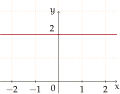
  Polynomial of degree 0:
  f(x) = 2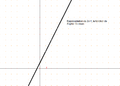

• 

  Polynomial of degree 1:
  f(x) = 2x + 1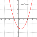

• 

  Polynomial of degree 2:
  f(x) = x² − x − 2
  = (x + 1)(x − 2)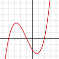

• 

  Polynomial of degree 3:
  f(x) = x³/4 + 3x²/4 − 3x/2 − 2
  = 1/4 (x + 4)(x + 1)(x − 2)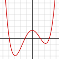

• 

  Polynomial of degree 4:
  f(x) = 1/14 (x + 4)(x + 1)(x − 1)(x − 3)
  + 0.5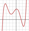

• 

  Polynomial of degree 5:
  f(x) = 1/20 (x + 4)(x + 2)(x + 1)(x − 1)
  (x − 3) + 2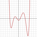

• 

  Polynomial of degree 6:
  f(x) = 1/100 (x⁶ − 2x ⁵ − 26x⁴ + 28x³
  + 145x² − 26x − 80)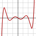

• 

  Polynomial of degree 7:
  f(x) = (x − 3)(x − 2)(x − 1)(x)(x + 1)(x + 2)
  (x + 3)

A polynomial function in one real variable can be represented by a graph.

• The graph of the zero polynomial
  f(x) = 0
  is the x-axis.
• The graph of a degree 0 polynomial
  f(x) = a₀, where a₀ ≠ 0,
  is a horizontal line with y-intercept a₀
• The graph of a degree 1 polynomial (or linear function)
  f(x) = a₀ + a₁x, where a₁ ≠ 0,
  is an oblique line with y-intercept a₀ and slope a₁.
• The graph of a degree 2 polynomial
  f(x) = a₀ + a₁x + a₂x², where a₂ ≠ 0
  is a parabola.
• The graph of a degree 3 polynomial
  f(x) = a₀ + a₁x + a₂x² + a₃x³, where a₃ ≠ 0
  is a cubic curve.
• The graph of any polynomial with degree 2 or greater
  f(x) = a₀ + a₁x + a₂x² + ⋯ + a_nxⁿ, where a_n ≠ 0 and n ≥ 2
  is a continuous non-linear curve.

A non-constant polynomial function tends to infinity when the variable increases indefinitely (in absolute value). If the degree is higher than one, the graph does not have any asymptote. It has two parabolic branches with vertical direction (one branch for positive x and one for negative x).

Polynomial graphs are analyzed in calculus using intercepts, slopes, concavity, and end behavior.

 المعادلات

المقالة الرئيسية: Algebraic equation

A polynomial equation, also called an algebraic equation, is an equation of the form

$$a_{n}x^{n}+a_{n-1}x^{n-1}+\cdots+a_{2}x^{2}+a_{1}x+a_{0}=0.$$

For example,

$$3x^{2}+4x-5=0$$

is a polynomial equation.

When considering equations, the indeterminates (variables) of polynomials are also called unknowns, and the solutions are the possible values of the unknowns for which the equality is true (in general more than one solution may exist). A polynomial equation stands in contrast to a polynomial identity like (x + y)(x − y) = x² − y², where both expressions represent the same polynomial in different forms, and as a consequence any evaluation of both members gives a valid equality.

In elementary algebra, methods such as the quadratic formula are taught for solving all first degree and second degree polynomial equations in one variable. There are also formulas for the cubic and quartic equations. For higher degrees, the Abel–Ruffini theorem asserts that there can not exist a general formula in radicals. However, root-finding algorithms may be used to find numerical approximations of the roots of a polynomial expression of any degree.

The number of solutions of a polynomial equation with real coefficients may not exceed the degree, and equals the degree when the complex solutions are counted with their multiplicity. This fact is called the fundamental theorem of algebra.

 Solving equations

المقالة الرئيسية: Algebraic equation

انظر أيضاً: Root-finding of polynomials and Properties of polynomial roots

A root of a nonzero univariate polynomial P is a value a of x such that P(a) = 0. In other words, a root of P is a solution of the polynomial equation P(x) = 0 or a zero of the polynomial function defined by P. In the case of the zero polynomial, every number is a zero of the corresponding function, and the concept of root is rarely considered.

A number a is a root of a polynomial P if and only if the linear polynomial x − a divides P, that is if there is another polynomial Q such that P = (x − a) Q. It may happen that a power (greater than 1) of x − a divides P; in this case, a is a multiple root of P, and otherwise a is a simple root of P. If P is a nonzero polynomial, there is a highest power m such that (x − a)^m divides P, which is called the multiplicity of a as a root of P. The number of roots of a nonzero polynomial P, counted with their respective multiplicities, cannot exceed the degree of P, and equals this degree if all complex roots are considered (this is a consequence of the fundamental theorem of algebra). The coefficients of a polynomial and its roots are related by Vieta's formulas.

Some polynomials, such as x² + 1, do not have any roots among the real numbers. If, however, the set of accepted solutions is expanded to the complex numbers, every non-constant polynomial has at least one root; this is the fundamental theorem of algebra. By successively dividing out factors x − a, one sees that any polynomial with complex coefficients can be written as a constant (its leading coefficient) times a product of such polynomial factors of degree 1; as a consequence, the number of (complex) roots counted with their multiplicities is exactly equal to the degree of the polynomial.

There may be several meanings of "solving an equation". One may want to express the solutions as explicit numbers; for example, the unique solution of 2x − 1 = 0 is 1/2. This is, in general, impossible for equations of degree greater than one, and, since the ancient times, mathematicians have searched to express the solutions as algebraic expressions; for example, the golden ratio ${\displaystyle{\displaystyle(1+{\sqrt{5}})/2}}$ is the unique positive solution of ${\displaystyle{\displaystyle x^{2}-x-1=0.}}$ In the ancient times, they succeeded only for degrees one and two. For quadratic equations, the quadratic formula provides such expressions of the solutions. Since the 16th century, similar formulas (using cube roots in addition to square roots), although much more complicated, are known for equations of degree three and four (see cubic equation and quartic equation). But formulas for degree 5 and higher eluded researchers for several centuries. In 1824, Niels Henrik Abel proved the striking result that there are equations of degree 5 whose solutions cannot be expressed by a (finite) formula, involving only arithmetic operations and radicals (see Abel–Ruffini theorem). In 1830, Évariste Galois proved that most equations of degree higher than four cannot be solved by radicals, and showed that for each equation, one may decide whether it is solvable by radicals, and, if it is, solve it. This result marked the start of Galois theory and group theory, two important branches of modern algebra. Galois himself noted that the computations implied by his method were impracticable. Nevertheless, formulas for solvable equations of degrees 5 and 6 have been published (see quintic function and sextic equation).

When there is no algebraic expression for the roots, and when such an algebraic expression exists but is too complicated to be useful, the unique way of solving it is to compute numerical approximations of the solutions. There are many methods for that; some are restricted to polynomials and others may apply to any continuous function. The most efficient algorithms allow solving easily (on a computer) polynomial equations of degree higher than 1,000 (see Root-finding algorithm).

For polynomials with more than one indeterminate, the combinations of values for the variables for which the polynomial function takes the value zero are generally called zeros instead of "roots". The study of the sets of zeros of polynomials is the object of algebraic geometry. For a set of polynomial equations with several unknowns, there are algorithms to decide whether they have a finite number of complex solutions, and, if this number is finite, for computing the solutions. See System of polynomial equations.

The special case where all the polynomials are of degree one is called a system of linear equations, for which another range of different solution methods exist, including the classical Gaussian elimination.

A polynomial equation for which one is interested only in the solutions which are integers is called a Diophantine equation. Solving Diophantine equations is generally a very hard task. It has been proved that there cannot be any general algorithm for solving them, or even for deciding whether the set of solutions is empty (see Hilbert's tenth problem). Some of the most famous problems that have been solved during the last fifty years are related to Diophantine equations, such as Fermat's Last Theorem.

 تعبيرات عديدة الحدود

Polynomials where indeterminates are substituted for some other mathematical objects are often considered, and sometimes have a special name.

 عديدات حدود مثلثية

المقالة الرئيسية: عديدة حدود مثلثية

A trigonometric polynomial is a finite linear combination of functions sin(nx) and cos(nx) with n taking on the values of one or more natural numbers. The coefficients may be taken as real numbers, for real-valued functions.

If sin(nx) and cos(nx) are expanded in terms of sin(x) and cos(x), a trigonometric polynomial becomes a polynomial in the two variables sin(x) and cos(x) (using the multiple-angle formulae). Conversely, every polynomial in sin(x) and cos(x) may be converted, with Product-to-sum identities, into a linear combination of functions sin(nx) and cos(nx). This equivalence explains why linear combinations are called polynomials.

For complex coefficients, there is no difference between such a function and a finite Fourier series.

Trigonometric polynomials are widely used, for example in trigonometric interpolation applied to the interpolation of periodic functions. They are also used in the discrete Fourier transform.

 عديدات حدود المصفوفات

المقالة الرئيسية: عديدة حدود المصفوفات

A matrix polynomial is a polynomial with square matrices as variables. Given an ordinary, scalar-valued polynomial

$$P(x)=\sum_{i=0}^{n}{a_{i}x^{i}}=a_{0}+a_{1}x+a_{2}x^{2}+\cdots+a_{n}x^{n},$$

this polynomial evaluated at a matrix A is

$$P(A)=\sum_{i=0}^{n}{a_{i}A^{i}}=a_{0}I+a_{1}A+a_{2}A^{2}+\cdots+a_{n}A^{n},$$

where I is the identity matrix.

A matrix polynomial equation is an equality between two matrix polynomials, which holds for the specific matrices in question. A matrix polynomial identity is a matrix polynomial equation which holds for all matrices A in a specified matrix ring M_n(R).

 عديدات الحدود الأسية

A bivariate polynomial where the second variable is substituted for an exponential function applied to the first variable, for example P(x, e^x), may be called an exponential polynomial.

 مفاهيم ذات صلة

 الدوال النسبية

المقالة الرئيسية: دالة نسبية

A rational fraction is the quotient (algebraic fraction) of two polynomials. Any algebraic expression that can be rewritten as a rational fraction is a rational function.

While polynomial functions are defined for all values of the variables, a rational function is defined only for the values of the variables for which the denominator is not zero.

The rational fractions include the Laurent polynomials, but do not limit denominators to powers of an indeterminate.

 عديدات حدود لوران

المقالة الرئيسية: متعددة حدود لوران

عديدات حدود لوران هي مثل عديدات الحدود، ولكنها تسمح بحدوث قوى سالبة للمتغيرات.

 متسلسلات القوى

المقالة الرئيسية: متسلسلة قوى شكلية

Formal power series are like polynomials, but allow infinitely many non-zero terms to occur, so that they do not have finite degree. Unlike polynomials they cannot in general be explicitly and fully written down (just like irrational numbers cannot), but the rules for manipulating their terms are the same as for polynomials. Non-formal power series also generalize polynomials, but the multiplication of two power series may not converge.

 حلقة عديدات الحدود

المقالة الرئيسية: حلقة عديدات الحدود

A polynomial f over a commutative ring R is a polynomial all of whose coefficients belong to R. It is straightforward to verify that the polynomials in a given set of indeterminates over R form a commutative ring, called the polynomial ring in these indeterminates, denoted ${\displaystyle{\displaystyle R[x]}}$ in the univariate case and ${\displaystyle{\displaystyle R[x_{1},\ldots,x_{n}]}}$ in the multivariate case.

One has

$$R[x_{1},\ldots,x_{n}]=\left(R[x_{1},\ldots,x_{n-1}]\right)[x_{n}].$$

So, most of the theory of the multivariate case can be reduced to an iterated univariate case.

The map from R to R[x] sending r to itself considered as a constant polynomial is an injective ring homomorphism, by which R is viewed as a subring of R[x]. In particular, R[x] is an algebra over R.

One can think of the ring R[x] as arising from R by adding one new element x to R, and extending in a minimal way to a ring in which x satisfies no other relations than the obligatory ones, plus commutation with all elements of R (that is xr = rx). To do this, one must add all powers of x and their linear combinations as well.

Formation of the polynomial ring, together with forming factor rings by factoring out ideals, are important tools for constructing new rings out of known ones. For instance, the ring (in fact field) of complex numbers, which can be constructed from the polynomial ring R[x] over the real numbers by factoring out the ideal of multiples of the polynomial x² + 1. Another example is the construction of finite fields, which proceeds similarly, starting out with the field of integers modulo some prime number as the coefficient ring R (see modular arithmetic).

If R is commutative, then one can associate with every polynomial P in R[x] a polynomial function f with domain and range equal to R. (More generally, one can take domain and range to be any same unital associative algebra over R.) One obtains the value f(r) by substitution of the value r for the symbol x in P. One reason to distinguish between polynomials and polynomial functions is that, over some rings, different polynomials may give rise to the same polynomial function (see Fermat's little theorem for an example where R is the integers modulo p). This is not the case when R is the real or complex numbers, whence the two concepts are not always distinguished in analysis. An even more important reason to distinguish between polynomials and polynomial functions is that many operations on polynomials (like Euclidean division) require looking at what a polynomial is composed of as an expression rather than evaluating it at some constant value for x.

 قابلية القسمة

المقالة الرئيسية: Polynomial greatest common divisor and Factorization of polynomials

If R is an integral domain and f and g are polynomials in R[x], it is said that f divides g or f is a divisor of g if there exists a polynomial q in R[x] such that f q = g. If ${\displaystyle{\displaystyle a\in R,}}$ then a is a root of f if and only ${\displaystyle{\displaystyle x-a}}$ divides f. In this case, the quotient can be computed using the polynomial long division.

If F is a field and f and g are polynomials in F[x] with g ≠ 0, then there exist unique polynomials q and r in F[x] with

$$f=q\,g+r$$

and such that the degree of r is smaller than the degree of g (using the convention that the polynomial 0 has a negative degree). The polynomials q and r are uniquely determined by f and g. This is called Euclidean division, division with remainder or polynomial long division and shows that the ring F[x] is a Euclidean domain.

Analogously, prime polynomials (more correctly, irreducible polynomials) can be defined as non-zero polynomials which cannot be factorized into the product of two non-constant polynomials. In the case of coefficients in a ring, "non-constant" must be replaced by "non-constant or non-unit" (both definitions agree in the case of coefficients in a field). Any polynomial may be decomposed into the product of an invertible constant by a product of irreducible polynomials. If the coefficients belong to a field or a unique factorization domain this decomposition is unique up to the order of the factors and the multiplication of any non-unit factor by a unit (and division of the unit factor by the same unit). When the coefficients belong to integers, rational numbers or a finite field, there are algorithms to test irreducibility and to compute the factorization into irreducible polynomials (see Factorization of polynomials). These algorithms are not practicable for hand-written computation, but are available in any computer algebra system. Eisenstein's criterion can also be used in some cases to determine irreducibility.

 انظر أيضاً

• Lill's method
• List of polynomial topics
• Polynomials on vector spaces
• متسلسلة أسية
• Table of mathematical expressions
• Polynomial transformations
• Polynomial mapping
• Polynomial functor

 المراجع

• Barbeau, E.J. (2003). Polynomials. Springer. ISBN 978-0-387-40627-5.
• Bronstein, Manuel; et al., eds. (2006). Solving Polynomial Equations: Foundations, Algorithms, and Applications. Springer. ISBN 978-3-540-27357-8.
• Cahen, Paul-Jean; Chabert, Jean-Luc (1997). Integer-Valued Polynomials. American Mathematical Society. ISBN 978-0-8218-0388-2.
• قالب:Lang Algebra. This classical book covers most of the content of this article.
• Leung, Kam-tim; et al. (1992). Polynomials and Equations. Hong Kong University Press. ISBN 9789622092716.
• Mayr, K. Über die Auflösung algebraischer Gleichungssysteme durch hypergeometrische Funktionen. Monatshefte für Mathematik und Physik vol. 45, (1937) pp. 280–313.
• Prasolov, Victor V. (2005). Polynomials. Springer. ISBN 978-3-642-04012-2.
• Sethuraman, B.A. (1997). "Polynomials". Rings, Fields, and Vector Spaces: An Introduction to Abstract Algebra Via Geometric Constructibility. Springer. ISBN 978-0-387-94848-5.
• Umemura, H. Solution of algebraic equations in terms of theta constants. In D. Mumford, Tata Lectures on Theta II, Progress in Mathematics 43, Birkhäuser, Boston, 1984.
• von Lindemann, F. Über die Auflösung der algebraischen Gleichungen durch transcendente Functionen. Nachrichten von der Königl. Gesellschaft der Wissenschaften, vol. 7, 1884. Polynomial solutions in terms of theta functions.
• von Lindemann, F. Über die Auflösung der algebraischen Gleichungen durch transcendente Functionen II. Nachrichten von der Königl. Gesellschaft der Wissenschaften und der Georg-Augusts-Universität zu Göttingen, 1892 edition.

 وصلات خارجية

• Hazewinkel, Michiel, ed. (2001), "Polynomial", Encyclopaedia of Mathematics, Kluwer Academic Publishers, ISBN 978-1556080104 
• "Euler's Investigations on the Roots of Equations". Archived from the original on September 24, 2012. {{cite web}}: Unknown parameter |deadurl= ignored (|url-status= suggested) (help)
• Eric W. Weisstein, Polynomial at MathWorld.

قالب:Polynomials